Efficient WaveRNN: Optimizing Nonlinearities
Implementing efficient nonlinearities for WaveRNN CPU inference is tricky but critical.
WaveRNN inference can be accelerated by using block-sparse weight matrices combined with specialized block-sparse matrix-vector multiplication kernels.
In this series of posts, we're going to go through the WaveRNN neural vocoder for audio waveform synthesis, along with a variety of implementation details and commonly used extensions. For a real implementation, check out the gibiansky/wavernn repository.
Posts in the Series:
As we reviewed in the previous blog post on WaveRNN inference, a single step of WaveRNN consists of sample embeddings, a GRU layer, two linear layers, and a sampling step.
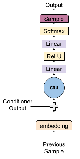
The bulk of the required compute (arithmetic) in this process can be grouped into four parts:
(As we saw in the previous post on WaveRNN inference, the GRU input-to-activation matrix can be accelerated by precomputing it and thus takes negligible compute.) Of these four steps, the first three (the matrix-vector multiplications) can be sped by replacing the matrices involved with sparse matrices.
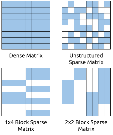
A sparse matrix is one where a significant proportion of its entries are zero. For example, a matrix with 90% sparsity has 90% of its entries filled with zeros. Since multiplying by zero produces zero, these entries contribute nothing to the overall final result. This means that if we know which entries are zero and don't bother computing with them, we can reduce the amount of compute by 10X and in theory realize a 10X speedup.
Of course, it's not that easy. In practice, efficient sparse matrix multiplication algorithms are very challenging to write and require high degrees of sparsity (>80%) to obtain any speedup, and the speedup they do obtain can be meager (for example, a 2X speedup for a matrix with 95% sparsity).
Sparse matrix multiplication algorithms are often slow due to the overhead of tracking which matrix entries are zeros and due to poor memory access patterns. For example, a simple sparse multiply can be implemented by storing a list of coordinates of non-zero entries and iterating over them to perform the multiplications and accumulations on those elements. However, if you load the coordinates from memory, then load the value at that coordinate from memory, then do the multiplication and accumulation, you end up doing two memory reads (one for the coordinates and one for the value) per multiplication – twice as many memory reads as a dense matrix multiply. Additionally, since you are accessing non-contiguous parts of your matrix, you will have a very unpredictable and cache-unfriendly memory access pattern. When benchmarked against dense matrix multiplies with optimized tiling for cache-friendly memory access implemented with vector instructions (AVX, SSE, NEON), a naive sparse matrix multiply will end up much slower up until ridiculous levels of sparsity and very large matrices.
Luckily, in deep learning (unlike in some other fields), we rarely care too much about the specific locations of the non-zero entries. We can train our neural networks to use any sparsity pattern we desire. Thus, we can use block sparsity to make our sparse matrix multiplication kernels much easier to write and much more efficient.
A block sparse matrix is a sparse matrix where entire blocks (a rectangular grid of values in the matrix) of the matrix are either zero or non-zero. With block sparsity, we only need to store the indices of non-zero blocks, which can be a significant reduction in the amount of indexing we need to perform (relative to unstructured sparsity).
Additionally, we can choose the block size so that we can use our processor's vector registers to do our arithmetic. Pretty much all modern processors support some sort of vector arithmetic. Vector instructions allow us to execute a single instruction to load, store, or perform arithmetic on multiple values at the same time, while still taking only one clock cycle (approximately). For instance, if our matrix block size is equal to our vector register length (e.g. 8 floats with AVX), we can implement simple kernels which load and multiply blocks as just a few instructions per block.
While block sparsity easily addresses the amount of indexing loading and arithmetic we need to do in our compute kernel, our memory access patterns can still be quite unfriendly to the cache. Since the non-zero blocks may be far away from each other in memory when the matrix is laid out densely, the memory accesses will not be on the same cache line. Additionally, the CPU prefetcher will not be able to predict access patterns and fetch the needed cache line in advance.
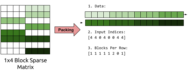
To improve our memory access patterns, we can repack our matrices in memory for easier access. For the purposes of WaveRNN inference, our matrix is fixed and we reuse it thousands of times, so the cost of repacking the matrix is negligible.
We can repack our matrix into a representation consisting of three arrays:

Our block sparse matrix-vector multiplication kernels can then read through these arrays start to finish in a linear pattern. Since we store only non-zero entries, our packed matrix might fit entirely in cache, and the prefetcher together with our linear access patterns can ensure that all our data has been loaded into the cache by the time we need it.
A simple algorithm for multiplying with these packed matrices (assuming 1x4 blocks) is to loop over the rows of the output vector. For each row, look up the number of blocks you need to multiply. For each block you need to multiply, read it from the data buffer, find the index its being multiplied by, read from that index, and perform your multiplication and accumulation. With this algorithm, the data buffer, the input indices, and the blocks per row are accessed in a completely predictable linear fashion, leading to good performance without much modification.
So far, we have discussed how to accelerate WaveRNN inference through switching out our dense matrix-vector multiplications for sparse (or block sparse) matrix-vector multiplications. To do so, we need to ensure that the weight matrices in the WaveRNN are primarily composed of zeros in a block sparse manner.
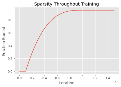
We can force our model to learn sparse weight matrices using magnitude-based weight pruning. During training, we identify the least important weights (as evidenced by their absolute value or magnitude) and then forcibly set them to zero. As training progresses, we snap progressively more and more weights to zero. Since the model starts out completely random, we allocate a bit of time (a warmup period) for the model to learn prior to beginning sparsification. The specific sparsification schedule used with WaveRNN is usually a cubic function which starts out rapidly pruning weights but, as the number of non-zero weights falls, slows down towards the end until it reaches its full expected level of sparsity.
To get a block-sparse matrix, instead of pruning individual weights based on their magnitude, we prune blocks, where the magnitude of a block is defined as the maximum magnitude of the weights in the block. We can implement sparsity by computing a block mask after every training iteration based on the block magnitudes and setting the weights to zero for the lowest magnitude weights.
Deep neural networks tend to be vastly overparameterized, and so the models learned this way with a very high degree of sparsity (90-95% sparse) are only slightly worse than dense models. However, training sparse models requires a long time – they take a very long time to converge.
A large fraction of WaveRNN inference time consists of matrix-vector multiplications. We can train deep neural networks which use sparse matrices – matrices which have a large fraction with zero entries. Since zero entries don't contribute to the final output, we can write highly efficient inference kernels for sparse matrix-vector multiplications speed up WaveRNN inference significantly. Sparse matrix-vector multiplications with unstructured sparsity (where non-zero entries are located anywhere) require very high levels of sparsity, but we can require block sparsity (where non-zero entries are contiguous in blocks) which allow for much more efficient memory access patterns and higher speedups. Block sparsity integrates well with vector instructions on modern processors (such as AVX and NEON instructions) which allow processing multiple values with a single instruction.
Check out the implementation at gibiansky/wavernn or proceed to the subsequent blog posts: