Efficient WaveRNN: Optimizing Nonlinearities
Implementing efficient nonlinearities for WaveRNN CPU inference is tricky but critical.
WaveRNN is an autoregressive neural vocoder, a neural network based process for converting low-dimensional acoustic features into an audio waveform by predicting the next sample in a stream of samples. Specialized compute kernels are necessary to make WaveRNN inference fast.
In this series of posts, we're going to go through the WaveRNN neural vocoder for audio waveform synthesis, along with a variety of implementation details and commonly used extensions. For a real implementation, check out the gibiansky/wavernn repository.
Posts in the Series:
WaveRNN is an autoregressive neural vocoder. Before diving into WaveRNN itself, let's break that statement down a bit.
A text-to-speech (TTS) system which converts text into spoken audio is comprised of many components. For instance, the frontend of a TTS engine converts input text to phonemes. Prosody and acoustic models assign durations to those phonemes and convert them into spectrograms (or equivalent acoustic features). Finally, a unit selection algorithm or a vocoder convert those acoustic features into an audio waveform. A neural vocoder is the last step in a speech synthesis pipeline.
To summarize, a neural vocoder is a neural network based algorithm for converting audio from an acoustic feature representation (such as log mel spectrograms) to a waveform.
(To synthesize audio, the spectrogram representation must already exist and have been created by another step in the TTS pipeline. WaveRNN alone cannot generate speech from text.)
There are many possible ways to build a neural vocoder – autoregressive models, GANs, invertible normalizing flows, diffusion models. Audio synthesis is one of the most well-studied areas of neural generative modeling, lagging only behind image synthesis.
An audio waveform consists of thousands of samples. Each sample is a single number corresponding to an instantaneous reading from a microphone. An autoregressive model (such as WaveRNN) generates a stream of audio by predicting the next sample given all previous samples and the spectrograms of nearby audio frames.
To generate audio, we start with an empty audio stream and predict the first sample. Using the first sample, we predict the second sample. Using the first and second samples, we predict the third sample. This continues until the entire waveform is generated. The spectrograms are an extra input to each of these predictions and guide all the predictions made by WaveRNN, which is trained to generate audio which corresponds to the spectrograms it is given.
In this section (and elsewhere), we assume that you are familiar with the basics of neural networks and deep learning. If not, grabbing a book (like this one or this one) may help.
WaveRNN consists of a few conceptual pieces:
The conditioning network can be run once on the entire input spectrogram, and the autoregressive network and sample embedding layer are alternated: a sample is generated, then prepared for the next timestep, then the next timestep is generated, and so on. At training time, though, the entire (real, non-synthesized) audio clip is available, and can be fed to the autogressive network, as shown below.
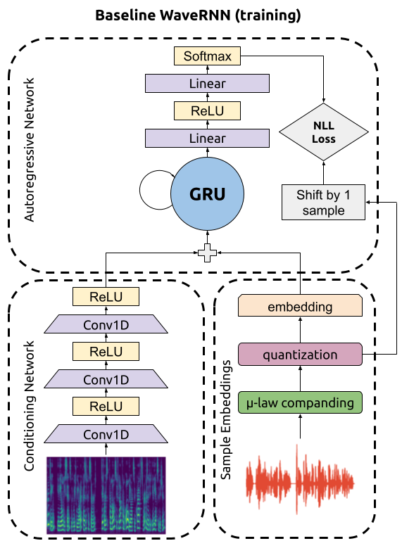
Audio waveforms are usually represented as a sequence of floating point numbers between -1 and 1. For WaveRNN, however, we apply two transformations to the audio waveform prior to using it:
(You could equivalently say that we discretize the range -1 to 1 into 256 different regions with regions far away from zero having an exponentially larger width than regions close to zero.)
For a given value $x$, µ-law companding maps it to $F(x)$ via
$$F(x) = \text{sgn}(x) \frac{\ln(1+ \mu |x|)}{\ln(1+\mu)}~~~~-1 \leq x \leq 1$$
As shown in this animation, companding stretches the example audio waveform scale, so that small variations near zero become big variations. The human ear is sensitive to the log of amplitude / intensity, so without this, the generated audio would be perceived as noisy.
The companded waveform is then converted to an integer (from 0 to 255) by subdividing the range -1 to 1 into equally spaced chunks. Mathematically, the quantization is done via $D(y)$ where
$$D(y) = \lfloor \frac{255}{2}(y + 1)+ \frac{1}{2}\rfloor.$$
We add $\frac{1}{2}$ so that zero (a common value in audio!) can be exactly mapped to the integer 128. You can verify that values near -1 will map to 0 and values near (but less than) 1 will map to 255.
Discretizing the audio waveform is crucial, because the way we predict the next audio sample is by treating the prediction as a multi-class classification problem. The network is trained to predict which class (from 0 to 255) the next audio sample falls in using a softmax cross entropy loss. To generate a sample, we sample from the multinomial distribution defined by the softmax probabilities.
To feed the audio samples into the autoregressive network, we convert them into sample embeddings by learning an embedding matrix with one row for each of the possible values. We can then obtain the input to the autoregressive network corresponding to an audio sample by looking at the corresponding row of the embedding matrix (that is, if the sample value is 193, we look at the 193rd value of the matrix and use that row as the input).
The input to a neural vocoder is a spectrogram or similar low-dimensional acoustic representation. A common choice is a log mel magnitude spectrogram. Let's briefly break that down!
Recall that a waveform can be represented as the sum of a large number of oscillating sine waves of varying frequencies and magnitudes. A magnitude spectrogram (computed via a short-time Fourier transform) indicates the power of the signal in each frequency band at a given time. In other words, a value in a spectrogram tells you the amplitude of the oscillating waves of a given frequency at a given time. A spectrogram looks like this:
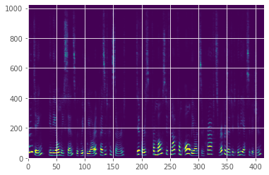
As mentioned earlier, human hearing is sensitive to the log of the power, which means that small differences near zero are as audible as large differences far away from zero. In this plot, it's hard to see those small differences, so instead we use a log spectrogram:
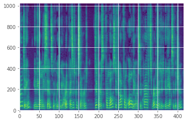
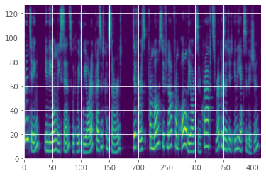
In addition to being sensitive to the log of power, human hearing is also sensitive to the log of frequency (pitch). High volumes in a narrow low frequency band near zero are as audible as high volumes spread throughout a wide high frequency band. To visualize this, we usually plot log mel magnitude spectrograms, as shown below. Mel spectrograms compress the frequency bands in a way that maps to human hearing.
The conditioning subnetwork of WaveRNN takes log mel spectrograms (or other low-dimensional acoustic features) as input, normalizes them (to be roughly -1 to 1 in magnitude), and then processes them with several layers of alternating convolutions and nonlinearities. It is crucial that the convolutions are non-causal and have both forwards and backwards context, as predicting the next sample at any given point depends not only on the audio sample history but also on the future spectrogram. Including the future context is what makes the spectrogram conditioning information helpful for next sample prediction and thus what causes WaveRNN to closely follow the spectrograms in its generated audio.
A single frame of the spectrogram corresponds to many samples. Depending on the hop length of the short-time Fourier transform used to compute the spectrogram, each frame of the spectrogram will correspond to dozens or hundreds of samples. Thus, the output of the final convolution and nonlinearity needs to be upsampled by a corresponding factor. For example, if a spectrogram frame is computed from a hop length of 256 samples, then each output timestep must be upsampled to 256 timesteps prior to being provided as input to WaveRNN.
The output of the conditioning network (post-upsampling) is a sequence of hidden layer output vectors, each vector corresponding to exactly one sample in the audio being synthesized.
The autoregressive network takes as input a sequence of sample embeddings and a sequence of conditioning vectors and uses them to predict the next sample in the sequence. This is done by:
The output of the softmax is a probability distribution. You can sample from that distribution to choose the next sample in the audio waveform.
To generate the full waveform, start by feeding the autoregressive network a sample corresponding to zero (assuming that most audio clips start with a bit of silence) and predicting the first sample. Then, feed the generated sample back to the autoregressive network to generate the second sample. Continue this process until the entire waveform is generated.
Since our audio is discretized, after the waveform is generated, the audio needs to be un-discretized and expanded (the opposite of companding is expanding) prior to being played back to the user.
Audio waveforms consist of many thousands of samples; a single second will usually contain between 16,000 samples (for 16 kHz audio) and 48,000 samples (for 48 kHz audio). This means that the GRU and linear layers must be run tens of thousands of times. This process is very computationally intense, and any non-computational overhead will result in it taking many seconds or even minutes to synthesize a short audio clip. In order to make WaveRNN usable for real-world applications, highly specialized and optimized implementations (compute kernels) are needed to make the synthesis process fast.
WaveRNN is an autoregressive neural vocoder. A neural vocoder is a neural network based process for converting low-dimensional acoustic features (such as log mel spectrograms) into an audio waveform. Autoregressive vocoders work by predicting the next sample in a stream of samples when given the acoustic features and all the previous samples. WaveRNN uses a discretized µ-law representation of audio to represent the audio as 8-bit integers and then predicts those values with a GRU, a fully connected layer, and a softmax layer, trained as a multi-class classification problem with a cross-entropy loss. Specialized compute kernels are necessary to make WaveRNN inference fast because an audio clip consists of tens or hundreds of thousands of samples, each of which require running a neural network to generate.
Check out the implementation at gibiansky/wavernn or proceed to the subsequent blog posts: