Efficient WaveRNN: Optimizing Nonlinearities
Implementing efficient nonlinearities for WaveRNN CPU inference is tricky but critical.
If implemented in Python and Pytorch, WaveRNN inference is too slow, but we can make it faster with several simple optimizations.
In this series of posts, we're going to go through the WaveRNN neural vocoder for audio waveform synthesis, along with a variety of implementation details and commonly used extensions. For a real implementation, check out the gibiansky/wavernn repository.
Posts in the Series:
As we discussed in the previous blog post, WaveRNN is an autoregressive neural vocoder which synthesizes audio sample-by-sample, as shown in the following diagram.
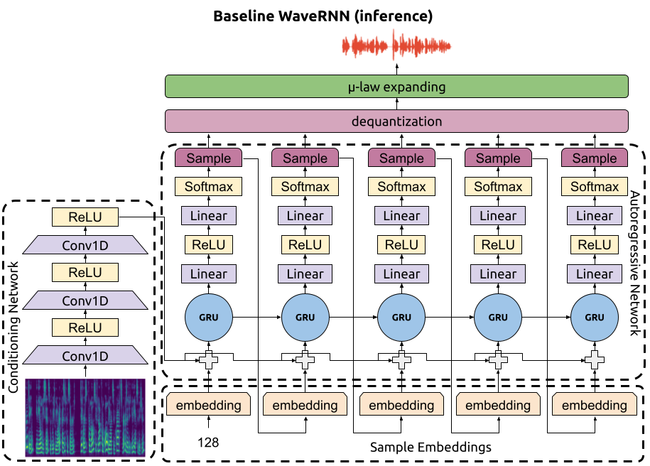
This means that after we run the conditioning network on the input spectrograms, we need to, for each sample:
Once the waveform is generated, dequantize the discretized samples and apply µ-law expanding to get the final waveform.
WaveRNN takes a lot of compute to run – for every synthesized sample, you need to run one timestep of the neural network. As a result, it can be quite slow to synthesize with. For interactive applications of TTS (such as voice assistants), you may want to start playing audio to the user before the entire synthesis is finished, which means you want to be able to stream through WaveRNN synthesis to minimize latency between receiving a TTS request and responding with initial synthesized audio.
To stream through the conditioning network, you can chunk up the input spectrograms into overlapping chunks and run those chunks separately through the network. (The chunks must be overlapping to avoid discontinuities at the boundaries; don't use zero padding when streaming through convolutions!) Alternatively, you can use a more clever approach to streaming through audio synthesis to avoid repeating computation in the conditioning network.
Streaming through the autoregressive network requires keeping track of two pieces of state: the previously synthesized sample (initialized to 128 representing zero) and the current GRU state (initialized to a vector of zeros). At each timestep, you run the autoregressive network to update the GRU state and generate a new sample.
Starting compute kernels generally has some overhead, so it is best to stream in chunks. A single invocation of the WaveRNN inference kernel should synthesize at least a few hundred samples (a few milliseconds of audio), and an outer loop should repeatedly call the inference kernel to synthesize the whole audio clip while sending intermediate results to the user.
Productionizing an implementation of WaveRNN requires a heavy focus on optimizing inference speed to achieve faster-than-realtime synthesis.
C++ Implementation: The first and largest optimization you can make is simply removing Python from the equation and implementing your inner inference loop in C++. For example in recent testing, using Python-based inference logic took about 100 seconds to synthesize 10 seconds of audio, but the same logic implemented in C++ (using the same matrix multiplication kernels, etc) took only 30 seconds (a roughly 3X speed-up). Implementing the kernel in C++ also opens the door to further optimizations, such as minimizing memory allocations, fine-grained multithreading, and more.
GRU Input Matrix Multiply Batching: Another optimization opportunity arises in the way GRUs are implemented. If you look at the PyTorch GRU implementation, we have two matrix multiplies: one that applies to the state and one that applies to the inputs.
$$\begin{align*}r_t &= \sigma(W_{ir} x_t + b_{ir} + W_{hr} h_{(t-1)} + b_{hr}) \\ z_t &= \sigma(W_{iz} x_t + b_{iz} + W_{hz} h_{(t-1)} + b_{hz}) \\ n_t &= \tanh(W_{in} x_t + b_{in} + r_t * (W_{hn} h_{(t-1)}+ b_{hn})) \\ h_t &= (1 - z_t) * n_t + z_t * h_{(t-1)}\end{align*}$$
For WaveRNN, the input is the sum of the conditioner network output $c_t$ (which changes once per frame) and the sample embedding $s_t$:
$$x_t = c_t + s_t.$$
We can compute a new sample embedding matrix which incorporates $W_{ir}$, $W_{iz}$, $W_{in}$, and their respective biases:
$$S = [W_{ir}; W_{iz}; W_{in}] s + [b_{ir}; b_{iz}; b_{in}].$$
We can also compute the product of the conditioner network $c_t$ with all these matrices. Since the conditioner network output is available in advance and only changes once per frame, we can batch these computations and do them once per frame outside the critical loop:
$$C = [W_{ir}; W_{iz}; W_{in}] c.$$
Then the GRU equations end up with one fewer matrix multiply:
$$\begin{align*}r_t &= \sigma(C_{rt} + S_{rt} + W_{hr} h_{(t-1)} + b_{hr}) \\ z_t &= \sigma(C_{zt} + S_{zt} + W_{hz} h_{(t-1)} + b_{hz}) \\ n_t &= \tanh(C_{nt} + S_{nt} + r_t * (W_{hn} h_{(t-1)}+ b_{hn})) \\ h_t &= (1 - z_t) * n_t + z_t * h_{(t-1)}\end{align*}$$
Implementing these optimizations leads to a 15-25% speedup, since you remove a significant fraction of the GRU layer compute from the inner loop.
Further Optimization: These optimizations are just the start and are insufficient for high quality synthesis at faster-than-realtime speeds. Further optimizations include block sparsity, int8 quantization, approximate nonlinearities, vector intrinsics (AVX-512, NEON, CUDA WMMA), multithreading, and so on.
The WaveRNN inference process consists of two distinct pieces: the conditioner network and the autoregressive inference. The conditioner network is simple and fast and can be implemented using standard PyTorch and Python tools. The autoregressive network runs once per audio sample and requires very heavy optimizations, starting with an implementation in C++. One straight forward optimization is batching the GRU input matrix multiply to reduce the amount of compute required for the GRU layer at each timestep. Many more inference optimizations are required to get a high quality faster-than-realtime neural vocoder.
Check out the implementation at gibiansky/wavernn or proceed to the subsequent blog posts: