Historically, fluid simulation methods have relied on a discretization of a 3-dimensional partial differential equation representing motion in a continuum. However, an alternative modern approach relies instead on viewing fluids from a statistical mechanics point of view, treating them as a set of particles with probability distributions on their locations and velocities and simulating the evolution of these distributions.
We begin by briefly deriving the Navier-Stokes equations for incompressible fluid flow; then, we take a look at an alternative approach via the Boltzmann transport equation; finally, we implement a discretization of the transport equation in a modern simulation technique known as the Lattice Boltzmann Method.
Navier Stokes Equations
The Navier-Stokes equations in their most basic form can be derived from a fairly simple physical standpoint, relying only on local conservation of mass and momentum. Extending the resulting equations to differnt fluids and circumstances requires substantial physical modeling, but the equations for Newtonian incompressible fluids are somewhat straightforward.
Local Consveration of Mass
First, consider the mass of fluid (of density $\rho({\bf x})$) within some control volume $\Omega$. The total mass within the volume is given by the integral $$M = \int_\Omega \rho({\bf x}) dV$$ As mass is conserved, we know that mass can only change via an influx or an outflux of fluid, which can occur either from a source or sink within the control volume or from flow in or out of the control volume. We can formalize this by expressing the derivative of $M$ with respect to time:
$$\frac{d}{dt} \int_\Omega \rho({\bf x}) dV = -\int_{\delta \Omega} \rho({\bf x}) {\bf v}\cdot {\bf n} d A - \int_\Omega Q d V$$
In the equation above, $Q$ represents a general source or sink term, which we can assume to be zero if we have no flow in or out of our system. The integral over the boundary $\delta \Omega$ represents the flow in or out of the boundary, and ${\bf v}$ is the velocity at ${\bf x}$. Applying the divergence theorem to the surface integral, we find that $$\frac{d}{dt} \int_\Omega \rho({\bf x}) dV = -\int_{\Omega}\nabla\cdot (\rho({\bf x}) {\bf v}) + QdV$$ If we flip the order of integration with the derivative, we find that we get the entire equation under the same integral, yielding $$ \int_\Omega \frac{d}{dt}\rho({\bf x}) +\nabla\cdot (\rho({\bf x}) {\bf v}) + QdV = 0$$ Since this applies to any control volume $\Omega$, the integrand itself must be zero; this assertion is equivalent to stating that mass must be locally conserved: $$\frac{d}{dt}\rho({\bf x}) +\nabla\cdot (\rho({\bf x}) {\bf v}) + Q = 0$$ If we assume no sources or sinks, we get a simple and elegant equation for the local conservation of mass: $$\dot{\rho} +\nabla\cdot (\rho {\bf v}) = 0$$
Local Conservation of Momentum
We begin by recalling Newton's third law relating force and acceleration: $${\bf F} = m {\bf a}.$$ We can put this in continuum form, expressing it with densities instead and assuming some "body force" $\bf b$: $${\bf b} = \rho({\bf x}) \frac{d}{dt}{\bf v}.$$ Next, expand the acceleration by substituting in the full derivative: $$\newcommand\p[2]{\frac{\partial #1}{\partial #2}} \newcommand\vv{{\bf v}} \frac{d}{dt}\vv = \p{\vv}{t} + \p{\vv}{x}\p{x}{t} + \p{\vv}{y}\p{y}{t} + \p{\vv}{z}\p{z}{t} = \p{\vv}{t} + \nabla \vv \cdot \vv$$ This yields the equation for local conservation of momentum: $${\bf b} = \rho\p{\vv}{t} + \rho\nabla \vv \cdot \vv.$$
Next Steps
We've derived a pair of equations for conservation of fluid mass and momentum: $$\begin{align*} \dot{\rho} +\nabla\cdot (\rho {\bf v}) &= 0 \\ \rho\p{\vv}{t} + \rho\nabla \vv \cdot \vv &= {\bf b} \end{align*}$$
While the central quantities of these equations, $\rho$ and $\bf v$, are easy to reason about intuitively, the forces acting on the fluid (represented by $\bf b$) are not so clear. Traditionally, the next step is an assumption about the set of body forces $\bf b$, followed by further simplifications; eventually, this reaches a point where the equation can be discretized in a clever manner and simulated. For Newtonian fluids, for instance, we assume that the body forces consist of some external force $\bf f$ and an internal fluid stress due to the pressure of the fluid. The resulting system is effectively a system of nonlinear partial differential equations of second order in seven dimensions (time, three space dimensions, and three velocity dimensions); simulating these accurately and efficiently is possible but quite difficult, and often causes numerical difficulties in addition to computational efficiency concerns. (For instance, naive implementations of incompressible fluid flow will introduce numerical errors that are indistinguishable from an extra viscosity term, even if it is assumed that the flow is entirely inviscid.)
Instead of delving into further details, we turn to the Boltzmann equation for a different approach.
Boltzmann Transport Equation
In this section, we provide a movitational sketch of a derivation for the Boltzmann transport equation. Note that we thoroughly ignore many physical aspects, focusing solely on the mathematics and nature of the differential equation. Developing physically accurate simulations would require a greater degree of attention to units and scaling constants, all of which we ignore.
The fundamental assumption behind the Boltzmann equation is that we can describe a system as a probability distribution over particles. Each particle has a probability density $f({\bf x}, {\bf v}, t)$ associated with it, which represents the probability that the particle is at position $\bf x$ with velocity $\bf v$ at time $t$. From this assumption, we can derive a collision-less variant of the Boltzmann transport equation.
Consider a particle of mass $m$ at position $\bf x$ at time $t$ with velocity $\bf v$. Assume also that some force $\bf F$ acts upon this particle. What, then, happens to this particle at time $t + \Delta t$? From basic Newtonian physics, we know that the particle will retain its mass $m$, but be at position ${\bf x} + \Delta t{\bf v}$ and have velocity ${\bf v} + \Delta t\frac{\bf F}{m}$. We can extend this reasoning to our probability density function and an infinitesimal time increment, $\Delta t = \delta t$: $$f({\bf x}, {\bf v}, t) = f\left({\bf x} + {\bf v}\delta t, {\bf v} + \frac{\bf F}{m}\delta t, t + \delta t\right)$$
We can use this to take the derivative, yielding
$$\lim_{\delta t \to 0} \frac{1}{\delta t}\left( f\left({\bf x} + {\bf v}\delta t, {\bf v} + \frac{\bf F}{m}\delta t, t + \delta t\right) -f({\bf x}, {\bf v}, t) \right) = 0.$$
We can obtain the same result via the chain rule, if we express $\bf x$ and $\bf v$ as functions of $t$. Evaluating this limit yields the equation
$$\newcommand\xx{{\bf x}} \begin{align*} \p{f}{t} + \p{f}{\xx}\p{\xx}{t} + \p{f}{\vv}\p{\vv}{t} &= \p{}{t}f + \p{\xx}{t}\cdot \nabla_\xx f + \p{\vv}{t}\cdot \nabla_\vv f \\ &= \left(\p{}{t} + \p{\xx}{t}\cdot \nabla_\xx+ \p{\vv}{t}\cdot \nabla_\vv\right)f \\ &= \left(\p{}{t} + \vv\cdot \nabla_\xx+ \frac{\bf F}{m}\cdot \nabla_\vv\right)f \\&= 0. \end{align*}$$
It is important to note that in our notation, $\nabla_\xx$ and $\nabla_\vv$ are not directional derivatives, buth rather simply shorthands for the gradient in the position and velocity spaces. Thus, we get our final collision-less Boltzmann transport equation: $$\left(\p{}{t} + \vv\cdot \nabla_\xx+ \frac{\bf F}{m}\cdot \nabla_\vv\right)f = 0.$$ To add in collisions, we do what we usually do when we want to add a driving force to a system that evolves as a particular differential equation – we change it from a homogenous to an inhomogenous equation. Thus, we posit that we can describe a Boltzmann equation with collisions using a collision operator $\Omega(t)$, yielding $$\left(\p{}{t} + \vv\cdot \nabla_\xx+ \frac{\bf F}{m}\cdot \nabla_\vv\right)f = \Omega(t).$$
Given this equation governing the microscopic dynamics of the system, we can derive macroscopic quantities of interest by integrating over $f$:
$$\begin{align*} \text{Density:}&\qquad\rho(\xx, t) &= \int f(\xx, \vv, t) d\vv \\ \text{Momentum:}&\qquad\rho(\xx, t) \vv &= \int \vv f(\xx, \vv, t) d\vv \\ \end{align*}$$
Discretization of the Boltzmann Equation
In order to simulate these equations, we must transform them into a set of algebraic equations via discretization. The Lattice Boltzmann Method is based on a somewhat strange discretization – we discretize time and space as usual onto a lattice with fixed width steps, and we discretize velocity into a finite number of potential directions. For example, for a two-dimensional setting, a common velocity discretization uses nine possible values, with $e_0$ corresponding to a zero velocity:
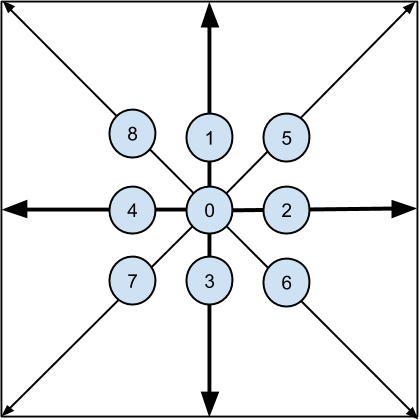
Consider now the final equation we arrived to: $$\left(\p{}{t} + \vv\cdot \nabla_\xx+ \frac{\bf F}{m}\cdot \nabla_\vv\right)f = \Omega(t).$$ In order to discretize it in the velocity space, consider what happens when we fix a velocity of interest, $\vv = e_i$, one of the nine directions shown above. Doing the substitution, we get $$\left(\p{}{t} + e_i \cdot \nabla_\xx+ \frac{\bf F}{m}\cdot \nabla_{\vv}\right)f = \Omega(t).$$ As we know from multivariable calculus, $e_i \cdot \nabla_{\xx} f$ is simply the directional derivative in the direction $e_i$; it is the rate of change of the quantity when we move in the direction indicated by $e_i$.
Next, consider the gradient in velocity space, $$\nabla_\vv f = \left(\p{f}{\vv_x}, \p{f}{\vv_y}, \p{f}{\vv_z}\right).$$ In order to proceed, we would need to evaluate $\nabla_\vv f(e_i)$, which we cannot do in generality. Thus, we assume that $\bf F$ is zero for the time being; there are several approaches to integrating body forces into the Lattice Boltzmann method, but they mostly group the body forces into the collision term, which we will deal with later.
Under this assumption, our equation reduces to $$\left(\p{}{t} + e_i \cdot \nabla_\xx\right)f = \Omega(t).$$ If we let $f_i$ be $f(\xx, e_i, t)$, this becomes $$f_i(\xx + e_i \delta t, t + \delta t) - f_i(\xx, t) = \Omega_i(t).$$
The collision term $\Omega$ is the last remaining bit, but it turns out to be incredibly complex in general. For the purposes of our simulation, we make a very common assumption known as the Bhatnagar-Gross-Krook (BGK) assumption: that the collision term simply forces the distribution to slowly decay to an equilibrium distribution $f^\text{eq}$, and thus that $$\Omega_i = \frac{1}{\tau}\left(f_i^\text{eq} - f_i\right).$$ The equilibrium distribution is effectively a smoothed version of the current distribution, recomputed from the bulk properties $\rho$ and $\bf u$ (bulk velocity). The equilibrium represents an expected distribution which would result in the observed bulk properties, and several assumptions are necessary to justify any particular form for $f^\text{eq}$. A commonly used form that was proposed for the BGK assumption is $$f_i^\text{eq} = \omega_i \rho \left(1 + 3\frac{e_i \cdot u}{c} + \frac92 \frac{(e_i \cdot u)^2}{c^2} - \frac32 \frac{u\cdot u}{c^2}\right).$$ where $\omega_i$ is a weighting function dependent on the exact velocity discretization.
Lattice Boltzmann Method Implementation
To implement the LBM method, we separate the solution of the equation $$f_i(\xx + e_i \delta t, t + \delta t) - f_i(\xx, t) = \Omega_i(t).$$ into two steps, referred to as streaming and collision steps. This approach is somewhat analogous to the common splitting mechanism used in solutions to the Navier-Stokes equations.
The streaming step takes care of fluid movement and propagation, the left side of the equation. As it does not deal with collisions, it can be done entirely separately for each of the discrete velocities, $e_i$. The distribution for a velocity $e_i$ at step $k+1$ for any grid point $\xx$ is computed by looking up the distribution at $\xx - e_i \Delta t$, which should just be one grid point away.
The streaming step is also where one must deal with some types of boundary conditions. The simplest type of boundary condition is simply the bounce-back boundary condition, that fluid incoming at a point hits a wall and bounces back. If the wall is at the edge of the fluid boundary, this is fairly simple. The fluid distribution with a velocity going away from the wall is determined not by some point beyond the wall (there is no fluid there!), but rather by the fluid coming into the wall with the opposite velocity.
After the streaming step, the collision step takes care of the $\Omega$ term. As we discussed earlier, the BGK approximation simply assumes that the net effect of all the collisions is to relax the distribution to some "equilibrium" distribution $f^\text{eq}$. Thus, the collision step is simply the computation of this equilibrium, along with the relaxation update $$f_i := f_i - \frac{1}{\tau}\left(f_i^\text{eq} - f_i\right).$$
To summarize, an implementation of the LBM method goes through the following steps:
- Initialization: Initialize a velocity distribution, $f_i$; then compute the initial equilibrium distribution, initial density, and initial velocity, as described previously.
- Streaming: Update each $f_i$ by propagating the fluid distribution in the direction $e_i$, applying bounce-back conditions as necessary.
- Collision: Compute the bulk properties density $\rho$ and velocity $\bf u$. Use these to compute the equilibrium distribution $f_i^\text{eq}$. Then, relax the fluid distribution to the equilibrium.
- Loop: Repeat streaming and collision indefinitely to simulate fluid motion.
The nice thing about the Lattice Boltzmann method is that it is easy to implement and almost trivially parallel, making it the perfect target for acceleration via GPUs and OpenCL/CUDA. A simple implementation I wrote in less than 300 lines is available on Github, yielding the following mesmerizing two-dimensional flows:
Conclusion
All in all, the Lattice Boltzmann method is a very interesting alternative to the traditional route of fluid simulation via discretization of the Navier-Stokes equations. On first glance, it seems that is is much less mathematically motivated; however, it seems like there are some very deep connections between the Boltzmann equation and the Navier-Stokes equations, which may be quite difficult to untangle. Others have managed to successfully relate (through a few assumptions about fluid behaviour) the Boltzmann transport equation to the Euler equations and the Navier-Stokes equations for incompressible fluid flow. However, understanding exactly why the Lattice Boltzmann method works as a suitable alternative to the Navier-Stokes equations requires some more work; in particular, it seems like creating physically-realistic flows for the purposes of engineering and simulation may be easier in a Navier-Stokes setting. Plenty of research has gone into these fields in the past ten years, so the papers are out there – but understanding them is a task for another day.