I've previously written about a number of machine learning techniques. However, when you first encounter a machine learning task, what do you try? Though neural networks and support vector machines and deep learning are very interesting and might make for great writing topics, Occam's razor tells us that really, we should be trying the simplest things first.

The simplest technique in machine learning is probably something very intuitive, something most people wouldn't even categorize as machine learning: \(k\)-Nearest Neighbor classification. Using a neural network for a problem where \(k\)-nearest neighbors would suffice, just because neural networks are more powerful in general, seems analogous to the classic problem of premature optimization. In other words, worth avoiding.

A \(k\)-nearest neighbor classifier is incredibly easy to describe: if you have a labeled data set \(\{x_i\}\), and you want to classify some new item \(y\), find the \(k\) elements in your data set that are closest to \(y\), and then somehow average their labels to get the label of \(y\).

In order to implement this, all you really need to do is answer two questions:

1. What is distance? Namely, if I have some \(x \in \{x_i\}\), how do I determine the distance from \(x\) to \(y\)?
2. If I know that \(x_1, x_2, \ldots, x_k\) are the \(k\) nearest neighbors of \(y\), how do I "average their labels"?

The answers to these questions depend greatly on exactly what you're dealing with. If you're dealing with textual data, then distance may be very hard to define; on the other hand, if you're dealing with points in a Cartesian coordinate system, we can immediately use our standard Euclidean distance as a distance metric. If your labels are real values (and your problem is a regression problem), then you can literally average them to get the label of \(y\); however, if your labels are classes, you may have to devise something more clever, such as letting the \(k\) neighbors vote on the label of \(y\).

Handwriting Recognition with k-Nearest Neighbors

Let's go ahead and implement \(k\)-nearest neighbors! Just like in the neural networks post, we'll use the MNIST handwritten digit database as a test set. You may be surprised at how well something as simple as \(k\)-nearest neighbors works on a dataset as complex as images of handwritten digits.

We'll start off with a generic class for doing \(k\)-nearest neighbors.

1
2
3
4
5
6
7
8
9
10
11
12
13
14
15
16
17
18
19
20
21
22
23
24
25
26
27
28
29

class NearestNeighborClassifier(object):
    """A generic k-nearest neighbor predictor.

    You need to extend this class and implement distance(from, to)
    and consensus(label_list) in order to make this functional."""
    
    def __init__(self, dataset, k):
        """Create a new nearest neighbor classifier.

        dataset - a list of data points. Each data point is an (x, y) pair,
                  where x is the input and y is the label.
        k - the number of neighbors to search for."""
        # Note how we don't have to do any initialization!
        # Once we have a dataset, we can immediately get predictions on new values.
        self.dataset = dataset
        self.k = k
        
    def predict(self, point):
        """Return the k-nearest neighbor prediction for a point."""
        # Compute distances to every point in the data set.
        distances = [self.distance(x[0], point) for x in self.dataset]
        
        # Naive approach: sort based on distances, take the first k elements.
        values = zip(distances, self.dataset)
        values.sort(key = lambda val: val[0])
        
        # Predict by averaging the closets k elements.
        prediction = self.consensus([value[1][1] for value in values[0:k]])
        return prediction

You'll immediately be able to notice two things. First of all, unlike many other models, we don't have any preliminary computations to do! There is no training phase in a \(k\)-nearest neighbor predictor; once we have the data set, we can make predictions. Also, this is a non-parametric model - we don't have any structure imposed on the predictor by some fixed parameter list, but instead the predictions are coming straight from the data.

The second thing you'll notice - possibly while cringing - is that the implementation above is terribly inefficient. If you have \(N\) training points in your data set, computing the distances to each point will take \(O(N)\) time, and then getting the first \(k\) values by sorting the data set based on distance will take another \(O(N \lg N)\) time, so you'll spend $O(N N) $ time for each prediction you want to make.

This is definitely suboptimal. We can improve this to \(O(kN)\) without much difficulty, simply by mimicking the first few steps of selection sort:

1
2
3
4
5
6
7
8
9
10
11
12
13
14
15
16
17
18
19
20
21
22
23
24
25

def predict(self, point):
    # We have to copy the data set list, because once we've located the best
    # candidate from it, we don't want to see that candidate again, so we'll delete it.
    candidates = self.dataset[:]
    
    # Loop until we've gotten all the neighbors we want.
    neighbors = []
    while len(neighbors) < self.k:
        # Compute distances to every candidate.
        distances = [self.distance(x[0], point) for x in candidates]
        
        # Find the minimum distance neighbor.
        best_distance = min(distances)
        index = distances.index(best_distance)
        neighbors.append(candidates[index])
        
        # Remove the neighbor from the candidates list.
        del candidates[index]
    
    # Predict by averaging the closets k elements.
    prediction = self.consensus([value[1] for value in neighbors])
    return prediction
        
# Let's go ahead and replace the old implementation.
NearestNeighborClassifier.predict = predict

This is still pretty terrible - if we're predicting thousands of points and have a large training data set, this can become pretty slow. But let's ignore that for now, and actually get something running! (There are ways to improve this runtime, but \(O(kN)\) is the best we can do without some pretty serious and very cool trickery.)

Reading the MNIST Image Database

We're going to have to deal with the ugly details of MNIST now. I'm providing the code below, but there's not much interesting to talk about.

1
2
3
4
5
6
7
8
9
10
11
12
13
14
15
16
17
18
19

import subprocess

def download(url):
    """Download a GZIP archive, return the data as a byte string."""
    # Do the download by shelling out to curl.
    cmd = 'curl "%s" | gzip -d' % url
    return subprocess.check_output(cmd, shell=True)

def get_files():
    """Download MNIST files from the internet."""
    url_format = "https://yann.lecun.com/exdb/mnist/%s-%s-idx%d-ubyte.gz"
    files = [("train", "images", 3), ("train", "labels", 1),
             ("t10k", "images", 3), ("t10k", "labels", 1)]
    
    urls = [url_format % values for values in files]
    data = [download(url) for url in urls]
    return data

data = get_files()

Now that we have the binary data, we can try to parse it. The file format used is pretty simple. Both the image and label files start with a 32-bit integer magic number, to verify integrity of the file. The next 32 bits are an integer letting us know how many samples there are in the file. After those two values, the label file contains unsigned bytes for each label. The image file has two more metadata integers (both 32 bits) representing the number of rows and columns in the images, and then just contains unsigned bytes for each pixel. (The images are black and white.)

This is ugly, but let's go ahead and parse these files. (For the record, I'm getting this information and magic numbers from here.)

1
2
3
4
5
6
7
8
9
10
11
12
13
14
15
16
17
18
19
20
21
22
23
24
25
26
27
28
29
30
31
32
33
34
35
36
37
38
39
40
41

import struct
from numpy import *

def parse_labels(data):
    """Parse labels from the binary file."""
    
    # We're going to use the Python 'struct' package. 
    # This is an incredibly nice package which allows us to specify the format
    # our data is in, and then automatically parses the data from the string.
    # Let's start by getting the magic number and the length: the first character
    # represents the endianness of the data (in our case, '>' for big endian), while
    # the next characters are the format string ('2i' for two integers).
    magic, n = struct.unpack_from('>2i', data)
    assert magic == 2049, "Wrong magic number: %d" % magic
    
    # Next, let's extract the labels.
    labels = struct.unpack_from('>%dB' % n, data, offset=8)
    return labels
    
def parse_images(data):
    """Parse images from the binary file."""
    
    # Parse metadata.
    magic, n, rows, cols = struct.unpack_from('>4i', data)
    assert magic == 2051, "Wrong magic number: %d" % magic
    
    # Get all the pixel intensity values.
    num_pixels = n * rows * cols
    pixels = struct.unpack_from('>%dB' % num_pixels, data, offset=16)
    
    # Convert this data to a NumPy array for ease of use.
    pixels = asarray(pixels, dtype=ubyte)
    
    # Reshape into actual images instead of a 1-D array of pixels.
    images = pixels.reshape((n, cols, rows))
    return images

train_images = parse_images(data[0])
train_labels = parse_labels(data[1])
test_images = parse_images(data[2])
test_labels = parse_labels(data[3])

Alright, we finally have our data in usable form. Let's look at it, by the way!

1
2
3
4
5
6
7
8
9
10
11
12
13
14

from matplotlib.pyplot import *

# Get the figure and axes.
fig, axes = subplots(5, 5)
axes = axes.reshape(25)
fig.suptitle("Random Sampling of MNIST")

# Plot random images.
indices = random.randint(len(train_images), size=25)
for axis, index in zip(axes, indices):
    image = train_images[index, :, :]
    axis.get_xaxis().set_visible(False)
    axis.get_yaxis().set_visible(False)
    axis.imshow(image, cmap = cm.Greys_r)

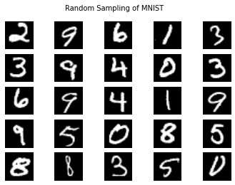
Looking good! Note that the MNIST database defines "0" to be white and "255" to be black. This is the opposite of what normal pixel intensities represent, which is why it's being displayed as white on black. But this doesn't matter for our purposes, so we'll just leave it be.

Classifying Handwritten Digits

Looking good! Alright, now let's finally answer those questions from the beginning of this post.

How are we going to define distance? It turns out there's definitely more than one way to define the distance between two images, and choosing the best one is crucial to good performance both in terms of accuracy and speed. But first, let's start with the simplest distance possible: Euclidean distance.

1
2
3
4
5
6
7

def euclidean_distance(img1, img2):
    # Since we're using NumPy arrays, all our operations are automatically vectorized.
    # A breakdown of this expression:
    #     img1 - img2 is the pixel-wise difference between the images
    #     (img1 - img2) ** 2 is the same thing, with each value squared
    #     sum((img1 - img2) ** 2) is the sum of the elements in the matrix.
    return sum((img1 - img2) ** 2)

One down, one to go. How are we going to take a consensus from all the \(k\) neighbors? This one is easy - just let them vote. Take the majority vote as the right answer!

1
2
3
4
5
6
7
8
9
10
11
12
13
14
15

from collections import defaultdict
def get_majority(votes):
    # For convenience, we're going to use a defaultdict.
    # This is just a dictionary where values are initialized to zero
    # if they don't exist.
    counter = defaultdict(int)
    for vote in votes:
        # If this weren't a defaultdict, this would error on new vote values.
        counter[vote] += 1
    
    # Find out who was the majority.
    majority_count = max(counter.values())
    for key, value in counter.items():
        if value == majority_count:
            return key

Alright, let's finally make our classifier and see how it does. We've done all the hard work, now just some boilerplate code.

1
2
3
4
5
6
7
8
9
10
11
12
13
14
15
16
17

# Create the predictor class.
class MNISTPredictor(NearestNeighborClassifier):
    def distance(self, p1, p2):
        return euclidean_distance(p1, p2)
    
    def consensus(self, values):
        return get_majority(values)
    
# Convert our data set into an easy format to use.
# This is a list of (x, y) pairs. x is an image, y is a label.
dataset = []
for i in xrange(len(train_images)):
    dataset.append((train_images[i, :, :], train_labels[i]))
    
# Create a predictor for various values of k.
ks = [1, 2, 3, 4, 5, 6]
predictors = [MNISTPredictor(dataset, k) for k in ks] 

Note that we haven't really put any thought into what \(k\) should be. Is one a good value? What about ten? What about a hundred? The greater \(k\), the better our predictions, right?

The true answer is that we don't know. The right way to find out is through a method called cross validation, but right now we can just take a look at how it does for several different values of \(k\).

1
2
3
4
5
6
7
8
9

def predict_test_set(predictor, test_set):
    """Compute the prediction for every element of the test set."""
    predictions = [predictor.predict(test_set[i, :, :]) 
                   for i in xrange(len(test_set))]
    return predictions

# Choose a subset of the test set. Otherwise this will never finish.
test_set = test_images[0:100, :, :]
all_predictions = [predict_test_set(predictor, test_set) for predictor in predictors]

Our classifier is way too slow to run the entire test set. Suppose we did want to run every image in of the ten thousand test images through the predictor. There are fifty thousand training images; so each prediction takes \(50000k\) image comparisons. We had values of \(k\) which summed to \(1 + 3 + 5 + 10 = 16\), so each prediction incurs 0.8 million image comparisons. Since we would have had ten thousand images, that would make for a total of eight billion image comparisons.

Suppose you had a 4 GHz CPU (I don't). And suppose that there was no overhead, and the only operations it had to do were the subtractions. Each image comparison incurs 28x28 operations, on the order of a thousand. That becomes a total of 8000 billion operations total, which, at 4 GHz, is slightly over half an hour. (I suspect this is about right, but we might be off by an order of magnitude. I wouldn't be surprised if it took four or five hours total.)

Evaluating Our Predictions

Let's see how we did. We can compute the accuracy by seeing what percentage each predictor got right.

1
2
3
4
5
6
7
8
9
10
11
12
13
14
15
16
17
18

def evaluate_prediction(predictions, answers):
    """Compute how many were identical in the answers and predictions,
    and divide this by the number of predictions to get a percentage."""
    correct = sum(asarray(predictions) == asarray(answers))
    total = float(prod(answers.shape))
    return correct / total

labels = asarray(test_labels[0:100])
accuracies = [evaluate_prediction(pred, labels) for pred in all_predictions]

# Draw the figure.
fig = figure(1)
plt.plot(ks, accuracies, 'ro', figure=fig)

fig.suptitle("Nearest Neighbor Classifier Accuracies")
fig.axes[0].set_xlabel("k (# of neighbors considered)")
fig.axes[0].set_ylabel("accuracy (% correct)");
fig.axes[0].axis([0, max(ks) + 1, 0, 1]);

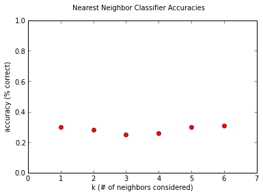
Surprisingly enough, it isn't terrible. Considering the chance of guessing randomly would be around 10%, our classifier is doing significantly better! But still, this is far from good, given the performance of neural networks in the previous post. It's interesting to note that the dependence on the value of \(k\) seems pretty weak, at least for the small values we're investigating. This is due to the pleasantly-named Curse of Dimensionality, which I might discuss sometime in the near future, as it's pretty much the reason that machine learning is Hard with a capital H.

There's a ton of stuff we could do to make this better. For our own convenience, we could start by parallelizing these operations, so we don't have to wait four hours for our results (if we have multiple CPUs). More interestingly, we could think of a better distance metric. For instance, we could use principal component analysis to project each image down to a lower-dimensional representation, and then use Euclidean distance in the lower dimensional space. We could also use a more intelligent neighbor-finding algorithm. These exist, but they aren't pretty, and have their own limitations to consider.

But those are for another blog post.