Efficient WaveRNN: Optimizing Nonlinearities
Implementing efficient nonlinearities for WaveRNN CPU inference is tricky but critical.

This is a continuation of Part 1 of this two-part series. In this post, I'll try to go over the implementation of PQMF filters in sufficient detail such that you'll be able to use this technique in your own code.
In the previous post, I summarized by presenting a recipe for converting a neural vocoder into a sub-band vocoder:
I left some of these pieces rather vague, and now it's time to fill in the details. Specifically, I'd like to address:
The bulk of this post will be addressing prototype filters, and we'll be using PyTorch for all code samples.
In this section, we'll dive into a prototype filter design method based on Kaiser windows.
Prior to jumping in, let's go over some vocabulary from filter design. For me, all of these rang bells from my signal processing classes years ago, but it was valuable to go through each of them.
tl; dr: You can do this with one call to scipy.signal.firwin
Given a window length $N$, Kaiser window filter $w(n)$ is the following:
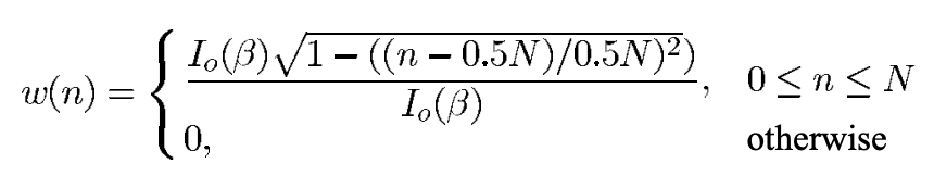
This defines a window of length $N+1$ using the modified Bessel function $I_0$ of the first kind. In practice, this can be computed using scipy.signal.windows.kaiser (which assumes $n$ is centered around zero by default).
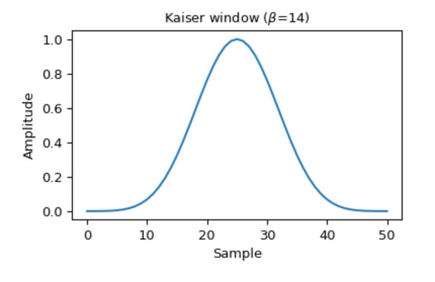
The Kaiser window looks like you'd expect a window to look like:
Given a stopband attenuation $As$ and transition bandwidth $\Delta w$, the filter length should be approximately:
$$N \approx \frac{As -7.95}{14.36\Delta w} 2\pi.$$
The derivation for this specific fact is supposedly available here, but I am for the time being willing to take this on faith. Similarly, the needed value for $\beta$ is also a function of your stopband attenuation $As$.
Given your chosen window function $w(n)$, your final prototype filter can be computed from your desired cutoff frequency $\omega_c$:
$$h(n) = \frac{\sin(\omega_c n) w(n)}{\pi n}.$$
We have yet to compute the cutoff frequency $\omega_c$, which, according to our reference paper, is best computed by minimizing the objective function
$$\phi_{\text{new}}(\omega_c) = \max |h(n) * h(N - n)|.$$
(That is, given an $\omega_c$, compute the prototype filter, convolve it with its reverse, and take the maximum absolute value. More details discussed here, but this seems to be right.)
For computing this in practice, you can use scipy.signal.firwin. firwin allows you to specify a window function; additionally, if you specify the width parameter, you can directly set the transition bandwidth and it will calculate the appropriate value of beta for your Kaiser window.
Now that we have a prototype filter computed using scipy.signal.firwin, we need to create a set of $K$ analysis filters $h_k(n)$ and synthesis filters $g_k(n)$. Recall from the previous post that these are defined as follows in PQMF filter banks:
$$\begin{align*}h_k[n] &= h[n] \cos\left(\frac{\pi}{4K}\left(2k + 1\right)\left(2n - N + 1\right) + \Phi_k\right)\\g_k[n] &= h_k[N - 1 - n]\\\Phi_k &= (-1)^{k} \frac{\pi}{4}.\end{align*}$$
Computing this is not too hard, just a bit of arithmetic. The process of using these filters is then equivalent to standard convolution.
With the math out of the way, let's convert this to code. Warning – don't copy this code and run it. I haven't tested it and I haven't run it, so it won't be useful to you that way. Instead, view this as a formalization of what I wrote above and trace through the logic to understand it.
def create_prototype_filter(bands: int, cutoff: float) -> np.ndarray:
    """Create a prototype filter."""
    transition_bandwidth = 0.9 * np.pi / 2 / bands
    attenuation = 100 # dB
    taps = int(2 * np.pi * (attenuation -7.95) / (14.36 * transition_bandwidth))
    return scipy.signal.firwin(
        taps, cutoff, width=transition_bandwidth, fs=2 * np.pi
    )

def optimize_cutoff(bands: int) -> float:
    """Choose the best cutoff frequency."""
    options = np.linspace(0.0, np.pi, 100000)
    best_cutoff, best_objective = None, 1e9
    for option in options:
        h = create_prototype_filter(bands, option)
        objective = np.abs(np.convolve(h, h[::-1])).max()
        if objective < best_objective:
            best_cutoff, best_objective = option, objective
    return best_cutoff

def create_filter_bank(bands: int):
    """Create the entire filter bank."""
    cutoff = optimize_cutoff(bands)
    proto = create_prototype_filter(bands, cutoff)
    taps = proto.size
    h = np.zeros((bands, taps))
    g = np.zeros((bands, taps))
    factor = (np.pi / (2 * bands)) * (
        np.arange(taps + 1) - ((taps - 1) / 2)
    )
    for k in range(bands):
        scale = (2 * k + 1) * factor
        phase = (-1) ** k * np.pi / 4
        h[k] = 2 * proto * np.cos(scale + phase)
        g[k] = 2 * proto * np.cos(scale - phase)

return h, gAll in all, as is often the case with mathematical ideas, the amount of code it takes to implement all of this is pretty small. Thank you additionally to @kan-bayashi who's Github repo was hugely helpful in tracing through some of the logic required.
This approach definitely raises additional questions, which I look forward to answering or seeing answered:
Definitely looking forward to seeing where all of this goes! I'm consistently impressed with the rapid progress in neural speech synthesis, so I'm sure the answers will come quickly.