Efficient WaveRNN: Optimizing Nonlinearities
Implementing efficient nonlinearities for WaveRNN CPU inference is tricky but critical.
In the past year or so, there's been several papers that investigate using sub-band coding with neural vocoders to model audio and accelerate inference:
In this blog post, I'd like to go over the ideas behind sub-band coding and specifically the math behind PQMF coding. You can find a more textbook-style approach to this in chapter 4 of this book (and, if you don't have a copy of this book or some of the above-linked papers, a wonderful person named Alexandra Elbakyan can likely help you).
When you work with audio, you can represent it in the time domain (as a waveform) or in the frequency domain (as a spectrogram). A spectrogram is obtained through a Discrete Fourier Transform, and tells you the power and phase of the audio at every frequency present in the audio.
The key idea behind sub-band coding is that instead of representing the audio as a single high-frequency (24kHz) signal that covers the entire range of frequencies, we can instead represent it as multiple lower-frequency (e.g. 6kHz) signals that cover ranges of frequencies (sub-bands).
We can use this alternate representation for different applications. In file compression (MP3), this is used to apply different levels of quantization and compression to the different bands (because human hearing is sensitive to them in different ways). In neural vocoding for TTS, we can use this to accelerate inference by having our neural vocoders output multiple sub-band values per output timestep, thus reducing the total amount of compute needed while keeping quality high.
Sub-band coding consists of two phases. In the first phase, analysis, the signal is processed with a set of $k$ analysis filters, creating $k$ new signals. These signals are downsampled by a factor of $k$ by taking every $k$th value (thus maintaining the same total amount of data). In audio compression applications, the downsampled signals are processed (quantization, compression, etc) and transmitted. The second phase, synthesis, reconstructs the original signal from the downsampled and processed signals. To reconstruct the original signal, the signals are then upsampled by a factor of $k$ to the original data rate by inserting $k - 1$ zeros after each value. These upsampled signals are processed with a set of $k$ synthesis filters (one filter per signal) and added together. If the analysis and synthesis filters are chosen appropriately, the output signal can either approximate or perfectly reconstruct the input signal.
For the application of neural vocoding, we apply the analysis filters to the training data and train our networks to produce all $k$ sub-band signals as outputs. We then apply synthesis to our network outputs to produce the final audio stream. This can accelerate inference over standard modeling techniques because the signal we are producing has been downsampled by a factor of $k$, and different bands for a single timestep are modeled as conditionally independently.
Next up, let's talk about the math behind sub-band coding.
We'll soon be talking a lot about discrete signal filters. A filter is a function that, given an input signal $x[t]$, produces a modified signal $y[t]$. Just like we use spectrograms to analyze audio signals in the frequency domain, analyzing the behavior of filters is commonly done in the frequency domain as well, and we use the Z transform (a discrete equivalent of a Laplace transform) to convert filters into the frequency domain.
Since the Z transform is a little less common than the discrete Fourier transform, it's worth going over. If you're familiar with it, skip to the next section.
The discrete Fourier transform of $x[n]$ is defined as:
$$X[f] = \sum_{n=0}^N x[n] e^{\frac{-i f n 2 \pi}{N}}.$$
The Z transform generalizes the $e^{\frac{i 2 \pi}{N}f}$ term to be any complex value $z$ instead of being restricted to the unit circle, and is defined as:
$$X[z] = \sum_{n=0}^\infty x[n] z^{-n}.$$
The Z transform has similar properties to the Fourier transforms. The relevant ones to our discussions are:
We will also need the Z transform for downsampling and upsampling (by dropping samples or inserting zeros):
If you need to, rederive the above properties to make sure they make sense to you!
Now that we have reviewed the Z transform, let's use it to analyze the synthesis and analysis processes and derive a set of filters for a pair of bands ($k=2$).
Consider the following diagram of analysis and synthesis (from Ch 4. of the aforementioned book):
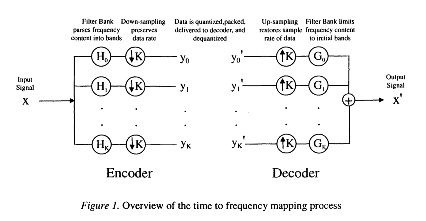
In our setup, we have analysis filters $H_0$ and $H_1$ and synthesis filters $G_0$ and $G_1$. The Z transform of $x'[n]$ (expressed using the transforms of the bands and the synthesis filters) is then:
$$X'[z] = Y_0(z^2) G_0(z) + Y_1(z^2) G_1(z).$$
This relies on two previously-discussed properties. First, passing a signal through a series of filters multiplies the filters', because applying a filter is convolving a signal with the filter's impulse response. Second, applying a time delay of 2 to a signal $Y_0(z)$ yields $Y_0(z^2)$, as mentioned above.
By the same general approach, we can write $Y_0(z)$ and $Y_1(z)$ using the analysis filters and the input signal:
$$Y_i(z) = \frac{1}{2}H_i(z^{1/2}) X[z^{1/2}] + \frac{1}{2}H_i(z^{-1/2}) X[z^{-1/2}].$$
Combining this, we can write $X'[z]$:
$$\begin{align*}X'[z] =& \frac{1}{2}X[z]\left(H_0(z)G_0(z) + H_1(z)G_1(z)\right) + \\ &\frac{1}{2}X[-z](H_0(-z)G_0(z) + H_1(-z)G_1(z)) \\ =& X[z].\end{align*}$$
To achieve perfect reconstruction, we need to choose filters such that $X'[z] = X[z].$ There are many possible filters that satisfy this.
One common choice of filters is a set of Quadrature Mirror Filters.
To motivate this choice, we first of all want to get rid of the $X[-z]$ term in the equation above (this term causes aliasing). We can do so by setting:
$$G_0(z) = -H_1(-z)\\G_1(z) = H_0(-z).$$
Plugging this in to the equation for $X'[z],$ we get:
$$X'[z] =\frac{1}{2}X[z](-H_0(z) H_1(-z) + H_1(z)H_0(-z)).$$
The QMF solution continues to simplify by setting $H_1(z) = -H_0(-z),$ so that
$$X'[z] =\frac{1}{2}X[z](H_0(z)^2 - H_0(-z)^2).$$
We can then choose any $H_0(z),$ as long as it satisfies:
$$H_0(z)^2 - H_0(-z)^2 = 2z^{-D}.$$
The factor of $z^{-D}$ allows us to create a delayed output signal.
One way to achieve this is using a 2-tap Haar filter. This filter has the impulse response
$$h_0[n] = \left\{\frac{1}{\sqrt{2}}, \frac{1}{\sqrt{2}}, 0, 0, \ldots\right\}.$$
To clarify, this means that $y[n] = \frac{1}{\sqrt{2}} (x[n] + x[n-1]).$ Using linearity and time delay properties, the Z transform of this Haar filter's impulse response is
$$H_0(z) = \frac{1}{\sqrt{2}}(1 + z^{-1}),$$
which we can verify meets the aforementioned constraint on $H_0(z)$.
From the equations we had earlier, we can drive all our analysis and synthesis filters:
$$\begin{align*}h_0[n] &= \left\{\frac{1}{\sqrt{2}}, \frac{1}{\sqrt{2}}, 0, 0, \ldots\right\}\\h_1[n] &= \left\{-\frac{1}{\sqrt{2}}, \frac{1}{\sqrt{2}}, 0, 0, \ldots\right\}\\g_0[n] &= \left\{\frac{1}{\sqrt{2}}, \frac{1}{\sqrt{2}}, 0, 0, \ldots\right\}\\g_1[n] &= \left\{\frac{1}{\sqrt{2}}, -\frac{1}{\sqrt{2}}, 0, 0, \ldots\right\}\end{align*}$$
With a bunch of arithmetic, you can verify that the output signal is indeed identical to the input signal.
While these filters do work mathematically, they end up being less useful in practice. For filters to be useful, you want them to separate the frequency domain neatly, such that each filter significantly attenuates frequencies outside its band and does not attenuate frequencies in its band. These Haar filters have incredibly wide bands, as shown below, and thus are not very useful:
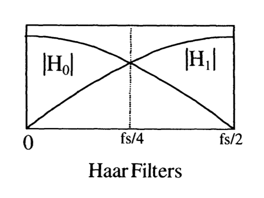
There exist better but approximate QMF solutions that have tighter frequency bands; these are longer (they have more than two taps).
The QMF filter bank works for two channels. However, in practice, we may want more than two channels. A generalization of the QMF filter bank to many channels exists, and is called the Pseudo-Quadrature Mirror Filter Bank (PQMF). These filters are called "pseudo-QMF" because these are approximate, not exact.
The filters used for DurIAN (see Appendix A) and MB-MelGAN are PQMF filters. These are created by following the methodology in "Near-Perfect-Reconstruction Pseudo-QMF Banks", and use four bands with a filter order of 63 (that is, have 63 "taps"). PQMF filter banks are also used in MP3 and other audio codecs.
PQMF filter banks consist of $K$ channels based on a low-pass filter $h[n]$. The $K$ analysis and synthesis filters are then computed from this chosen low-pass filter as follows:
$$\begin{align*}h_k[n] &= h[n] \cos\left(\frac{\pi}{4K}\left(2k + 1\right)\left(2n - N + 1\right) + \Phi_k\right)\\g_k[n] &= h_k[N - 1 - n]\end{align*}$$
The analysis filters $h_k[n]$ are cosine-modulated versions of the original filter (making PQMF filters part of a class of filters known as Cosine-Modulated Filter Banks or CMFBs). The synthesis filter is a time-reversed version of the analysis filter. Additionally, the cosine phases of adjacent bands are constrained and must satisfy (for integral $r$)
$$\Phi_k - \Phi_{k-1} = \frac{\pi}{2}(2r + 1).$$
One option, recommended in Eq. 11 here, is the following choice:
$$\Phi_k = (-1)^{k} \frac{\pi}{4}.$$
We can verify that this indeed meets the criterion above.
The choice of the prototype low-pass filter $h[n]$ is important for reducing reconstruction error. In fact, this filter can be found using computational methods by optimizing an objective function which minimizes the magnitude of the reconstruction error and maximizes stopband attenuation.
One approach to computationally designing the prototype filter is presented here; another approach based on limiting the search to Kaiser windows is available here. The latter approach seems significantly simpler to understand and easier to implement.
Finally, let's summarize the approach into a series of steps we can take to modify any neural vocoder with sub-band coding.
As some meta-commentary, I'm fascinated that this clever idea took such a long time to reach neural vocoders, and I suspect that now that it's been shown to be effective in several works, it will spread quickly. This seems like a classic case of slow progress due to siloed knowledge: the people with the deep understanding of MPEG filter banks for the most part were unlikely to be training neural vocoders, and the people training neural vocoders were unlikely to have deep knowledge of MPEG filter banks. It took several skilled and cross-functional researchers to make this happen – at least one person to have the initial idea, and then several more to reproduce it in several more works to get wider acclaim for this idea. This also really highlights how valuable domain experience can be – you can't dive into a new field, sprinkle some machine learning fairy dust, and get great results!